Scatterplots

%matplotlib inline
import matplotlib.pyplot as plt, numpy as np # import statements

squares = [1,4,9,16,25] # dataset for y axis
inputs = [1,2,3,4,5] # dataset for x axis

fig, ax = plt.subplots() # figure for new plot
ax.scatter(inputs, squares, s=100) # generate plot with custom dot size

ax.set_title("Square Numbers") # set plot title
ax.set_xlabel("Value") # set x axis label
ax.set_ylabel("Square of Value") # set y axis label

plt.show() # show output

fig, ax = plt.subplots() # figure for new plot
ax.scatter(inputs, squares, marker='x') # generate plot with custom marker

ax.set_title("Square Numbers") # set plot title
ax.set_xlabel("Value") # set x axis label
ax.set_ylabel("Square of Value") # set y axis label

plt.show() # show output

For more on scatterplots:

• matplotlib, “Scatter plot”

• matplotlib, “Scatter Demo2”

• matplotlib.pyplot.scatter

• Jake VanderPlas, “Simple Scatter Plots” from Python Data Science Handbook

Histograms

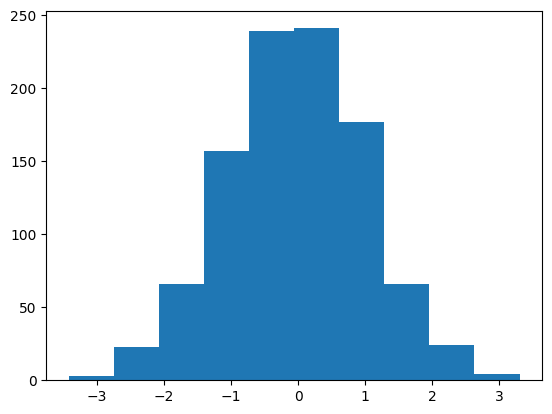
A histogram is a type of plot that approximates the distribution of numerical data.

• The first step in constructing a histogram is to bin or bucket the range of values. In other words, we need to divide the entire range of values into a series of intervals.

• The second step in constructing a histogram is to count how many values fall into each interval.

In a histogram, the bins are usually consecutive, non-overlapping intervals. The bins must be adjacent and are often (but not necessarily) of equal size.

data = np.random.randn(1000) # create randomized dataset
fig, ax = plt.subplots() # create figure
ax.hist(data) # create histogram with default bins
plt.show() # show output

Additional Resources

For more on histograms:

• matplotlib “Some features of the histogram (hist) function”

• matplotlib, “Histograms”

• matplotlib.pyplot.hist

• Jake VanderPlas, “Histograms, Binnings, and Density” from Python Data Science Handbook

Bar Charts

One of the common uses for bar charts is to plot categorial variables. A bar chart presents categorical data with rectangular bars with heights or lengths proportional to the values they represent.

# basic vertical bar chart

data = {'apple': 10, 'orange': 15, 'lemon': 5, 'lime': 20} # dictionary with categories and amounts
names = list(data.keys()) # get category names
values = list(data.values()) # get values
fig, axs = plt.subplots() # create figure
axs.bar(names, values) # create plot
plt.show() # show output

# horizontal bar chart
data = {'apple': 10, 'orange': 15, 'lemon': 5, 'lime': 20} # dictionary with categories and amounts
names = list(data.keys()) # get category names
values = list(data.values()) # get values
fig, axs = plt.subplots() # create figure
axs.barh(names, values) # create plot
plt.show() # show output

Additional Resources

For more on bar charts and plotting categorical data:

• matplotlib, Plotting categorical variables

• matplotlib, Horizontal bar chart

• matplotlib, Stacked bar chart

• matplotlib, Percentiles as horizontal bar chart

Categorical Data

This kind of categorical data can be plotted different ways, depending on the type of data and purpose or intent for the visualization. For example, we could plot the fruit data from the previous example as a bar chart, scatter plot, and line plot. An example of those three types side-by-side:

data = {'apple': 10, 'orange': 15, 'lemon': 5, 'lime': 20} # dictionary with categories and amounts
names = list(data.keys()) # get category names
values = list(data.values()) # get values

fig, axs = plt.subplots(1, 3, figsize=(9, 3), sharey=True) # create figure with 3 subplots

axs[0].bar(names, values, color='red') # bar chart
axs[1].scatter(names, values, color='green') # scatter plot
axs[2].plot(names, values) # line plot

fig.suptitle('Categorical Plotting') # figure title
plt.show() # show output